Stellar Population Continuum
This section describes how to simulate stellar continuum spectra using the spec1d.StellarContinuum module in GEHONG.
Stellar Population Templates
The simulation is based on a grid of single stellar population (SSP) templates, currently adopted from the EMILES library.
These templates are managed by the StellarContinuumTemplate class, which loads and prepares the template cube.
Required Input:
config: AConfiginstance that defines the wavelength grid.pathname: Path to EMILES template files (optional; default is provided).
Usage Example:
from gehong import spec1d
stellar_tem = spec1d.StellarContinuumTemplate(config)
Stellar Continuum Spectrum Generation
The StellarContinuum class synthesizes the stellar continuum spectrum using either single-population or composite star formation models.
Two working modes are supported:
Magnitude-calibrated mode (empirical flux scaling)
Triggered when mag is provided. The input sfh and ceh can be scalars (single SSP) or arrays (for composite populations).
Parameters:
mag: SDSS r-band magnitude.sfh: Star formation history. Scalar (age in Gyr) or array [[age, SFR]].ceh: Metallicity history. Scalar ([Fe/H] in dex) or array [[age, [Fe/H]]].vel: Line-of-sight velocity (km/s).vdisp: Velocity dispersion (km/s).ebv: Dust extinction E(B-V).
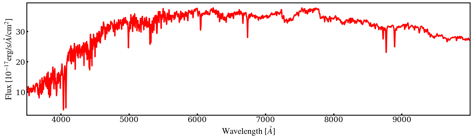
Example (single SSP):
stellar = spec1d.StellarContinuum(config, stellar_tem,
                                  mag=17.5, sfh=5.0, ceh=-0.3,
                                  vel=8000, vdisp=120, ebv=0.1)
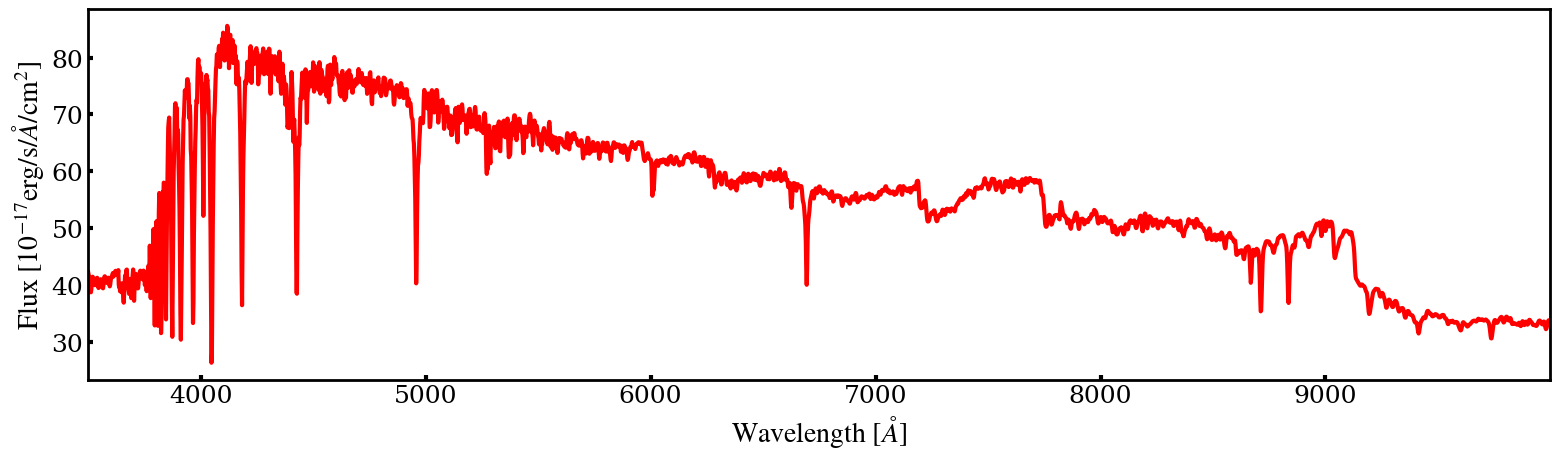
Example (composite SFH with magnitude scaling):
import numpy as np

# Define a typical galaxy SFH and CEH
age_grid = np.linspace(0.05, 13.7, 50)  # Gyr
sfh = np.exp(-age_grid / 3.0)           # τ = 3 Gyr exponential decay
ceh = -1.0 + (age_grid / np.max(age_grid)) * 1.0  # [Fe/H] from -1.0 to 0.0

# Combine into [age, value] arrays
sfh_array = np.column_stack((age_grid, sfh))
ceh_array = np.column_stack((age_grid, ceh))

stellar = spec1d.StellarContinuum(config, stellar_tem,
                                mag=17.0,
                                sfh=sfh_array,
                                ceh=ceh_array,
                                vel=6000, vdisp=100, ebv=0.15)
In this example, the final spectrum shape is determined by the SFH and CEH arrays, while the total flux is normalized to match an r-band magnitude of 17.0.
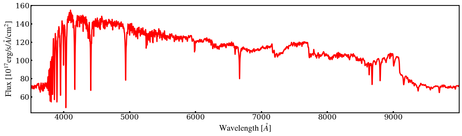
Physically-calibrated mode (flux from SFH)
Triggered when mag is set to None. In this mode, sfh and ceh must be 2D arrays.
Parameters:
sfh: Array of [[age (Gyr), SFR (M☉/yr)]].ceh: Array of [[age (Gyr), [Fe/H] (dex)]].z: Redshift.vpec: Peculiar velocity (km/s).vdisp: Velocity dispersion (km/s).ebv: Dust extinction E(B-V).
Example:
stellar = spec1d.StellarContinuum(config, stellar_tem,
                                  sfh=sfh_array,
                                  ceh=ceh_array,
                                  z=0.015, vpec=300, vdisp=100, ebv=0.2,
                                  mag=None)
Output Attributes
stellar.wave: 1D wavelength array in Ångströms.stellar.flux: Corresponding flux array in units of \(10^{-17}\ \mathrm{erg\ s^{-1}\ cm^{-2}\ Å^{-1}}\).
Note
In physical mode, the output flux is computed from SFH normalization and cosmological distance. In magnitude-calibrated mode, flux is normalized to the input magnitude.
StellarContinuum supports both empirical and physical modeling of galaxy spectra, with consistent units and interface across modes.