Two-Dimensional Map
To simulate IFS data of extended sources (e.g., galaxies), a set of two-dimensional (2D) physical parameter maps is required. These maps are classified into two major categories:
Stellar Component Maps: describing the distributions of stellar properties used to construct stellar continuum spectra (see Section Stellar Continuum Spectrum). These include maps of surface brightness, stellar age, and stellar metallicity. All these maps are handled by the
map2d.StellarPopulationMapmodule.Gas Component Maps: describing the distributions related to ionized gas, including those used to simulate emission-line spectra (see Section Ionized Gas Emission Lines). These include the \(\text{H}\alpha\) flux map, gas-phase metallicity, etc., and are combined via the
map2d.IonizedGasMapmodule.
Each map module accepts two-dimensional arrays as inputs and constructs pixel-by-pixel spectral components based on the corresponding physical parameters. To ensure consistency, all maps are aligned in coordinate system and shape. The Map2D class provides utility functions for rotating, shifting, or reprojecting maps as needed.
In addition to model-based generation, all modules support importing observational or simulation-based data cubes as custom maps. This enables flexible hybrid modeling combining empirical and analytic inputs.
To achieve realistic IFS simulations, the physical maps should exhibit detailed spatial structures, as illustrated in following Figure. Ideally, such maps are derived from real high-resolution observations or hydrodynamic simulations. As a practical alternative, we provide a set of parametric 2D models:
map2d.sersic_mapfor surface brightness profiles;map2d.tanh_mapfor velocity fields;map2d.gred_mapfor parameter gradients (e.g., age, metallicity).
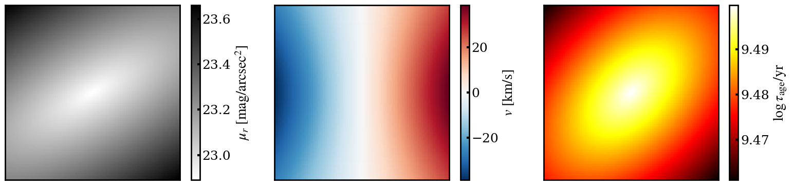
图 1 Example of three types of parametric 2D model maps used in GEHONG: Sersic brightness profile, rotation velocity field, and radial gradients.
StellarPopulationMap
The StellarPopulationMap class combines multiple 2D maps describing stellar properties to simulate the stellar continuum in each spaxel.
Two operating modes are supported:
Magnitude-Calibrated Mode: If a surface brightness map (
sb) is provided, the output spectrum is normalized using the given r-band magnitude. The age and metallicity maps only determine the spectral shape, not its normalization.Physically Calibrated Mode: If
sbis not provided, the spectrum is generated from physically motivated quantities including star formation history (SFH), metallicity, redshift, and peculiar velocity. This mode produces absolute flux calibrated spectra.
The stellar population at each position may be modeled using either a single stellar population (SSP) or a composite one defined via SFH and chemical enrichment history (CEH).
IonizedGasMap
The IonizedGasMap class generates emission-line spectra for ionized gas (HII regions) at each spatial position, based on key physical parameters such as Hα luminosity, gas-phase metallicity, velocity dispersion, and dust extinction.
Two modes are supported:
Flux-Calibrated Mode: If a 2D Hα map is given, it is used to scale the total emission-line luminosity.
Physically Derived Mode: If Hα is not given, it is derived from the input star formation rate, redshift, and metallicity, consistent with standard ionizing photon production models.
This module internally calls the HII_Region class to generate the emission-line spectrum at each pixel.
Sérsic Model
The surface brightness distribution of galaxies is modeled by a 2D Sérsic profile (Sérsic 1963, Graham et al. 2005):
where:
\(I_e\) is the surface brightness at the effective radius \(R_e\) (
reff),\(n\) is the Sérsic index (
n), controlling the concentration,\(b_n\) is a function of \(n\), defined by:
\[\Gamma(2n)=2\gamma(2n, b_n)\]\(R(x, y)\) is the elliptical radius from the galaxy center \((x_0, y_0)\), calculated as:
\[R(x, y) = \sqrt{R_\text{maj}^2(x, y) + \left (\frac{R_\text{min}(x, y)}{q}\right )^2}\]with:
\[\begin{split}R_\text{maj}(x, y) = (x - x_0) \cos \theta + (y - y_0) \sin \theta \\ R_\text{min}(x, y) = -(x - x_0) \sin \theta + (y - y_0) \cos \theta\end{split}\]\(q = b/a\) is the axis ratio (
ellip = 1 - q),\(\theta\) is the position angle (
pa).
For flux calibration, the model uses the total magnitude \(m_\text{tot}\) (mag) to derive the total luminosity:
Tanh Velocity Model
The map2d.tanh_map module models the velocity field assuming an axisymmetric rotation curve:
where:
\(i = \arccos (1-q)\) is the inclination angle,
\(\phi\) is the azimuthal angle, defined as:
\[\cos \phi = \frac{-(x-x_0)\,\sin \theta+(y-y_0)\,\cos \theta}{R(x, y)}\]\(V_c(R)\) is the rotational velocity curve defined by:
\[V_c(R) = V_\text{max} \tanh(R/R_t)\]where
vmaxis the asymptotic velocity andrtis the turnover radius (van der Kruit & Allen 1978, Andersen & Bershady 2003).
Gradient Model
Other stellar and gas parameters (e.g., age, metallicity) are commonly modeled using a logarithmic radial gradient profile via map2d.gred_map:
where:
\(A_\text{eff}\) (
aeff) is the parameter value at \(R_e\),\(\nabla_A\) (
gred) is the logarithmic gradient of parameter \(A\).
This model is supported by observations of galaxies (e.g., Koleva et al. 2011, Sánchez-Blázquez et al. 2014).