Mocking Two-Dimensional Map
This simulation is implemented by the map2d module.
Initialization of Two - Dimensional Images
In the gehong package, all two-dimensional distributions are passed in the form of a class based
on map2d.Map2d(). Therefore, it is necessary to initialize it before simulating a two-dimensional distribution.
Main Input Parameters:
Simulation data configuration class:
config
Usage Example:
To simulate a surface brightness distribution, you need to create a class for this two-dimensional distribution first. For example:
from gehong import map2d
sbmap = map2d.Map2d(config)
Non-Parameterized Two-Dimensional Distributions
The gehong package allows you to directly import existing two-dimensional distributions of
physical parameters (such as observational results and numerical simulation results) into the Map2d class.
For example, if you know the velocity field vmap of a galaxy, which is in the form of a two-dimensional array as follows:
[
    [-60.10162265, -59.73061567, -59.35098406,..., -5.27919182, -4.79226447, -4.31059388],
    [-59.57527736, -59.20481535, -58.82573166,..., -4.756253, -4.26990175, -3.78884127],
    [-59.0411374, -58.67117677, -58.29259928,..., -4.2276208, -3.74189254, -3.26148904],
   ...,
    [3.26148904, 3.74189254, 4.2276208,..., 58.29259928, 58.67117677, 59.0411374],
    [3.78884127, 4.26990175, 4.756253,..., 58.82573166, 59.20481535, 59.57527736],
    [4.31059388, 4.79226447, 5.27919182,..., 59.35098406, 59.73061567, 60.10162265]
]
You can import the above two-dimensional array using the .loadmap() method of the Map2d class. For example:
velmap = map2d.Map(config)
velmap.loadmap(vmap)
The imported two-dimensional distribution is stored in the attribute .map. You can check it like this:
print(velmap.map)

[
    [-60.10162265, -59.73061567, -59.35098406,..., -5.27919182, -4.79226447, -4.31059388],
    [-59.57527736, -59.20481535, -58.82573166,..., -4.756253, -4.26990175, -3.78884127],
    [-59.0411374, -58.67117677, -58.29259928,..., -4.2276208, -3.74189254, -3.26148904],
   ...,
    [3.26148904, 3.74189254, 4.2276208,..., 58.29259928, 58.67117677, 59.0411374],
    [3.78884127, 4.26990175, 4.756253,..., 58.82573166, 59.20481535, 59.57527736],
    [4.31059388, 4.79226447, 5.27919182,..., 59.35098406, 59.73061567, 60.10162265]
]
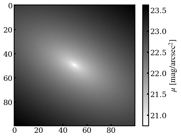
Sersic Model
The method .sersic_map() of the Map2d class can be used to simulate a two-dimensional surface brightness
distribution of the Sersic model.
Input Parameters:
mag: Integrated magnitude of the Sersic model, Unit: \(\text{mag}\), Range: 8 mag to 26 mag.r_eff: Effective radius, Unit: \(\text{arcsec}\), Range: greater than 0 arcsec.n: Sersic index, Unit: None. Parameter range: greater than 0.ellip: Ellipticity. Unit: None. Parameter range: 0 <= ellip < 1.theta: Position angle. Unit: \(\text{degree}\), Parameter range: - 180° to 180°.
Attributes:
- .map: Simulated two - dimensional distribution, Unit: \(\text{mag/arcsec}^2\).
Usage Example:
sbmap.sersic_map(mag = 15.0, r_eff = 4.0, n = 1.0, ellip = 0.2, theta = - 30)
This code will simulate a two - dimensional Sersic distribution with a total magnitude of \(15 \text{mag}\), an effective radius of \(4.0\text{arcsec}\), a Sersic index of 1, an ellipticity of 0.2, and a position angle of \(- 30\text{degree}$\).
The simulated two - dimensional distribution is as follows:
Tanh Velocity Field Model
The method .tanh_map() of the Map2d class can be used to simulate a velocity field where
the rotation curve is based on the tanh function.
Input Parameters:
vmax: Maximum rotation velocity, Unit: \(\text{km/s}\). Parameter range: > 0 \(\text{km}\ \text{s}^{-1}\).rt: Turnover radius of the rotation curve. Unit: \(\text{arcsec}\). Parameter range: > 0 arcsec.ellip: Ellipticity. Unit: None. Parameter range: 0 <= ellip < 1.theta: Position angle. Unit: \(\text{degree}\), Parameter range: - 180° to 180°.
Attributes:
.map: Simulated two - dimensional distribution. Unit: \(\text{km/s}\).
Usage Example
velmap = map2d.Map2d(config)
velmap.tanh_map(vmax=160, rt=2.0, ellip=0.5, theta=30)
This code will simulate a velocity field with a maximum rotation velocity of \(160 \text{km/s}\), a turnover radius of the rotation curve of \(2.0\text{arcsec}\), an ellipticity of \(0.5\), and a position angle of \(30\text{degree}\).
The simulated two - dimensional distribution is as follows:

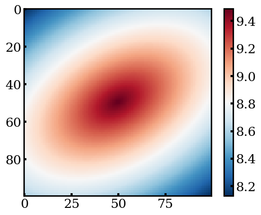
Two - Dimensional Gradient Model
The method .gred_map() of the Map2d class can be used to simulate a two - dimensional distribution
based on a gradient model.
Input Parameters:
a0: Central intensity. Unitless, with no specific parameter range.r_eff: Effective radius. Unit: \(\text{arcsec}\), and the parameter range is greater than 0 arcsec.gred: Gradient. Unit: \(\text{arcsec}^{-1}\), with no specific parameter range.ellip: Ellipticity. Unit: None. Parameter range: 0 <= ellip < 1.theta: Position angle. Unit: \(\text{degree}\), Parameter range: - 180° to 180°.
Attributes:
Simulated two - dimensional distribution (
.map): Unitless.
Usage Example:
agemap = m.Map2d(config)
agemap.gred_map(a0 = 9.5, r_eff = 1, gred = -1.2, ellip = 0.4, theta = 30)
This code will simulate a two - dimensional distribution with a central intensity of \(9.5\), an effective radius of \(1.0\text{arcsec}\), a gradient of \(-1.2\), an ellipticity of \(0.4\), and a position angle of \(30\text{degree}\).
The simulated two - dimensional distribution is as follows: